
This post transcribes to the hypertext and dead format the interactive tutorial and custom extensions shipped with the PharoPDS library to explore and understand Bloom filters.
So, if you want to start tinkering with these data structures in a really live environment, try to install the library in a Pharo image and follow the interactive tutorials or play with the custom tools provided.
Understanding Bloom filters
A Bloom filter is a space-efficient data structure, conceived by Burton Howard Bloom in 1970 (Space/Time Tradeoffs in Hash Coding with Allowable Errors), that represents a set of elements and allows you to test if an element is a membership.
A regular hash-based search stores the full set of values from a collection in a hash table, whether in linked lists or using open addressing. In both cases, as more elements are added to the hash table, the time to locate an element increases, degenerating the expected time performance from the initial constant O(1) to the lineal O(N).
A Bloom filter provides an alternative structure that ensures constant performance, both in space and time, when adding elements or checking an element membership. This behaviour is independent of the number of items already added to the filter.
The price paid for this efficiency is that a Bloom filter is a probabilistic data structure. As Bloom explains in his seminal paper:
The new methods are intended to reduce the amount of space required to contain the hash-coded information from that associated with conventional methods. The reduction in space is accomplished by exploiting the possibility that a small fraction of errors of commission may be tolerable in some applications, in particular, applications in which a large amount of data is involved and a core resident hash area is consequently not feasible using conventional methods.
Context
Donald Knuth in his famous The Art of Computer Programming writes the following about Bloom filters:
Imagine a search application with a large database in which no calculation needs to be done if the search was unsucessful. For example, we might want to check somebody’s credit rating or passport number, and if no record for that person appears in the file we don’t have to investigate further. Similarly in an application to computerized typesetting, we might have a simple algorithm that hyphenates most words correctly, but it fails on some 50,000 exception words; if we don’t find the word in the exception file we are free to use the simple algorithm.
Also Andrei Broder and Michael Mitzenmacher established the known as The Bloom Filter Principle (Network Applications of Bloom Filters: A Survey):
Wherever a list or set is used, and space is at a premium, consider using a Bloom filter if the effect of false positives can be mitigated.
Examples from the Real World™
- Medium uses Bloom filters to avoid recommending articles a user has previously read.
- Google Chrome uses a Bloom filter to identify malicious URLs.
- Google BigTable, Apache HBase and Apache Cassandra use Bloom filters to reduce the disk lookups for non-existing rows or columns.
- The Squid Web proxy uses Bloom filters for cache digests.
Basic understanding
The Bloom Filter can store a large set very efficiently by discarding the identity of the elements; i.e. it stores only a set of bits corresponding to some number of hash functions that are applied to each added element by the algorithm.
Practically, the Bloom Filter is represented by a bit array and can be described by its length (m) and number of different hash functions (k).
The structure supports only two operations:
- Adding an element into the set, and
- Testing whether an element is or is not a member of the set.
The Bloom Filter data structure is an array of bits where at the beginning all bits are equal to zero, meaning the filter is empty.
For example, consider the following Bloom filter example created to represent a set of 10 elements with a false positive probability (FPP) of 0.1 (i.e. 10%).
This empty filter will be backed by a bit array of length m=48 (storageSize) and 4 hash functions to produce values in the range {1, 2, ..., m}. It has the following form:
emptyBloomFilter
    <gtExample>
    | bloom |
    bloom := PDSBloomFilter new: 10 fpp: 0.1.
    self assert: bloom size equals: 0.
    self assert: bloom hashes equals: 4.
    self assert: bloom storageSize equals: 48.
    ^ bloom
Inspector on an empty Bloom filter showing the array of bits
To insert an element x into the filter, for every hash function hi we compute its value j=hi(x) on the element x and set the corresponding bit j in the filter to one.
As an example, we are going to insert some names of cities into the previous filter. Let’s start with the String 'Madrid':
withMadridBloomFilter
    <gtExample>
    | bloom |
    bloom := self emptyBloomFilter.
    bloom add: 'Madrid' asByteArray.
    self assert: bloom size equals: 1.
    ^ bloom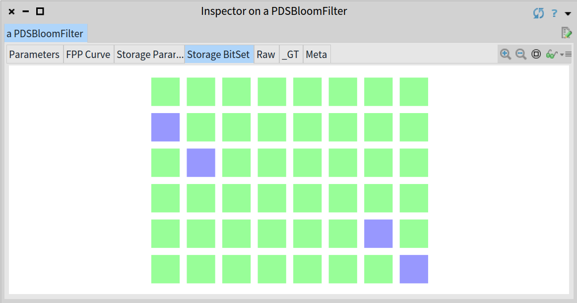
Inspector on the Bloom filter once added 'Madrid' showing 4 bits set
In order to find the corresponding bits to be set for 'Madrid', the filter computes the corresponding 4 hash values. As you see above, the filter has set the bits 9, 18, 39 and 48.
It is possible that different elements can share bits, for instance, let’s add another city, 'Barcelona', to the same filter:
Inspector on the Bloom filter showing 7 bits set after adding 'Madrid' and 'Barcelona'
As you can see, after adding the String 'Barcelona' to the previous Bloom filter only the bits 30, 36 and 42 have been set, meaning that the elements 'Madrid' and 'Barcelona' share one of their corresponding bits.
To test if a given element x is in the filter, all k hash functions are computed and the bits in the corresponding positions are checked. If all bits are set, then the element x may exist in the filter. Otherwise, the element x is definitely not in the filter.
The uncertainty about the element’s existence originates from the possibility of situations when some bits are set by different elements added previously.
Consider the previous Bloom filter example with the elements 'Madrid' and 'Barcelona' already added. To test if the element 'Barcelona' is a member, the filter computes its 4 hash values and checks that the corresponding bits in the filter are set, therefore the String 'Barcelona' may exist in the filter and the contains: 'Barcelona' returns true:
1withMadridAndBarcelonaCheckBarcelonaBloomFilter
2 <gtExample>
3 | bloom |
4 bloom := self withMadridBloomFilter.
5 blomm add: 'Barcelona' asByteArray.
6 self assert: bloom size equals: 2.
7 self assert: (bloom contains: 'Barcelona' asByteArray).
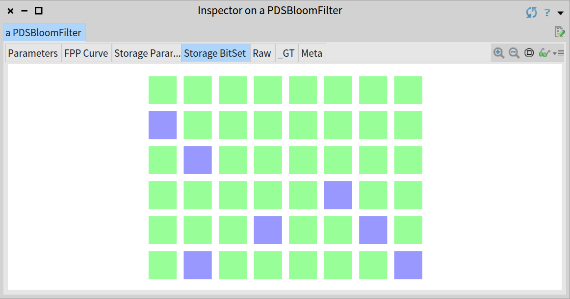
8 ^ bloomNow if we check the element 'Berlin', the filter computes its hashes in order to find that the corresponding bits in the filter are the following:
withBerlinBloomFilter
    <gtExample>
      | bloom |
      bloom := self emptyBloomFilter.
      bloom add: 'Berlin' asByteArray.
      self assert: bloom size equals: 1.
      ^ bloom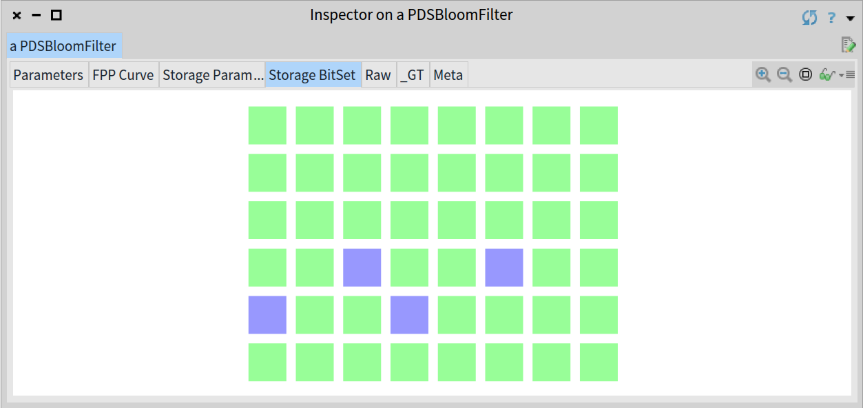
Inspector on the Bloom filter after adding the String 'Berlin'
We see that the bits 27 and 33 aren’t set, therefore the 'Berlin' element is definitely not in the filter, so the contains: method returns false:
1withMadridAndBarcelonaCheckBerlinBloomFilter
2    <gtExample>
3    | bloom |
4    bloom := self withMadridBloomFilter.
5    bloom add: 'Barcelona' asByteArray.
6    self assert: bloom size equals: 2.
7    self assert: (bloom contains: 'Berlin' asByteArray) not.
8    ^ bloom
A Bloom filter can also result in a false positive. For example, consider the element 'Roma', whose 4 hash values collision in the bit 36 that is already set in our filter example, so the contains: method concludes the element may exist in the filter:
1
2withMadridAndBarcelonaCheckRomaBloomFilter
3    <gtExample>
4      | bloom |
5      bloom := self withMadridBloomFilter.
6      bloom add: 'Barcelona' asByteArray.
7      self assert: bloom size equals: 2.
8      self assert: (bloom contains: 'Roma' asByteArray).
9      ^ bloom
As we know, we have not added that element to the filter, so this is an example of a false positive event. In this particular case, the bit 36 was set previously by the 'Barcelona’ element.
Properties
False positives
As we have shown, Bloom filters can lead to situations where some element is not a member, but the algorithm returns it might be. Such an event is called a false positive and can occur because of hard hash collisions or coincidence in the stored bits of different elements. In the test operation there is no knowledge of whether the particular bit has been set by the same hash function as the one we compare with.
Fortunately, a Bloom filter has a predictable false positive probability (FPP):
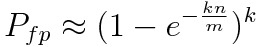
False positive probability for a Bloom filter
where n is the number of values already added, k the number of hashes and m the length of the filter (i.e. the bit array size).
In the extreme case, when the filter is full, every lookup will yield a (false) positive response. It means that the choice of m depends on the estimated number of elements n that are expected to be added, and m should be quite large compared to n.
In practice, the length of the filter m, under given false positive probability FPP and the expected number of elements n, can be determined by the formula:
Optimal length for a Bloom filter given an expected FPP
For the given ratio of m/n, meaning the number of allocated bits per element, the false positive probability can be tuned by choosing the number of hash functions k. The optimal choice of k is computed by minimizing the probability of false positives with the following formula:
Optimal number of different hash functions for a Bloom filter
Our PDSBloomFilter implementation is built specifying the estimated number of elements to be added (n) and the false positive probability (FPP), then the data structure uses the previous formula to compute the optimal number of hashes and bit array length.
For instance, to handle 1 billion elements and keep the probability of false positive events at about 2% we need the following Bloom filter:
oneBillionBloomFilter
    <gtExample>
      | bloom |
      bloom := PDSBloomFilter new: 1000000000 fpp: 0.02.
      self assert: bloom size equals: 0.
      self assert: bloom hashes equals: 6.
      self assert: bloom storageSize equals: 8142363337.
      ^ bloom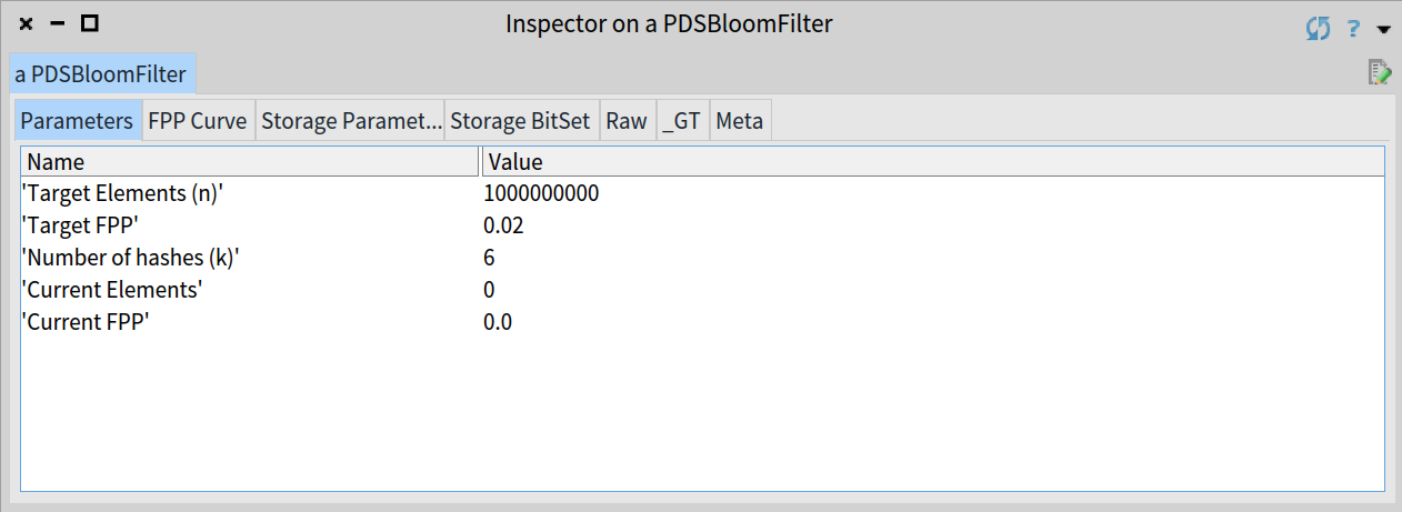
Parameters for the previous Bloom filter able to handle 1 billion elements with FPP equal to 2%
As you can see, the optimal number of hashes is 6 and the filter’s length is 8.14 x 109 bits, that is approximately 1 GB of memory.
False negatives
If the Bloom filter returns that a particular element isn’t a member, then it’s definitely not a member of the set.
Deletion is not possible
To delete a particular element from the Bloom filter it would need to unset its corresponding k bits in the bit array. Unfortunately, a single bit could correspond to multiple elements due to hash collisions and shared bits between elements.
Analysis
The previous formula for the false positive probability is a reasonably computation assuming the k hash functions are uniformly random.
By other hand, the fpp value specified when the PDSBloomFilter is initialized should be interpreted as the desired fpp once the expected n elements have been added to the structure.
For example, for a just created and still empty Bloom filter the data structure will have a fpp equal to 0, as you can see in the graph below:
The FPP for an empty filter is equals to 0
As you add elements to the filter the fpp is increased and will be equal to the target fpp when the filter reach the expected number of elements, as we can see if we fill the Bloom filter:
fullBloomFilter
    <gtExample>
    | bloom |
    bloom := self emptyBloomFilter.
    1 to: bloom targetElements
        do: [ :each | bloom add: each asString asByteArray ].
    ^ bloom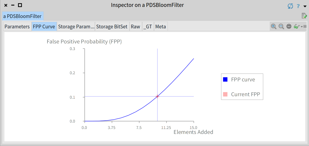
The estimated FPP will be equal to the established value when the filter contains the number of expected elements n
Nevertheless, you should know that the previous FPP curve is a theoretical value and the actual FPP observed will depend on the specific dataset and hash functions you work with. In order to check empirically the goodness of our implementation we have run the following analysis:
- Randomly generate a list of email addresses and insert them in the Bloom filter.
- Randomly generate a list of email addresses not inserted in the filter.
- Count the false positive events when searching for the missing addresses in the filter.
We ran the experiment for values from 10 to 1.5 times the expected number of elements in the filter (with steps of 10). For each number of elements the experiment is ran 10 times. The analysis shows a graph depicting the theoretical FPP curve of the filter (blue line), the average FPP values measured in each experiment (grey crosses), the actual FPP curve (red line) and the standard deviation (red shade).
For instance, the following code runs the previous empirical analysis and shows a graph with the results for a Bloom filter with 100 elements and FPP equal to 3%:
PDSBloomFilterAnalysis openFor: (PDSBloomFilter new: 100 fpp: 0.03)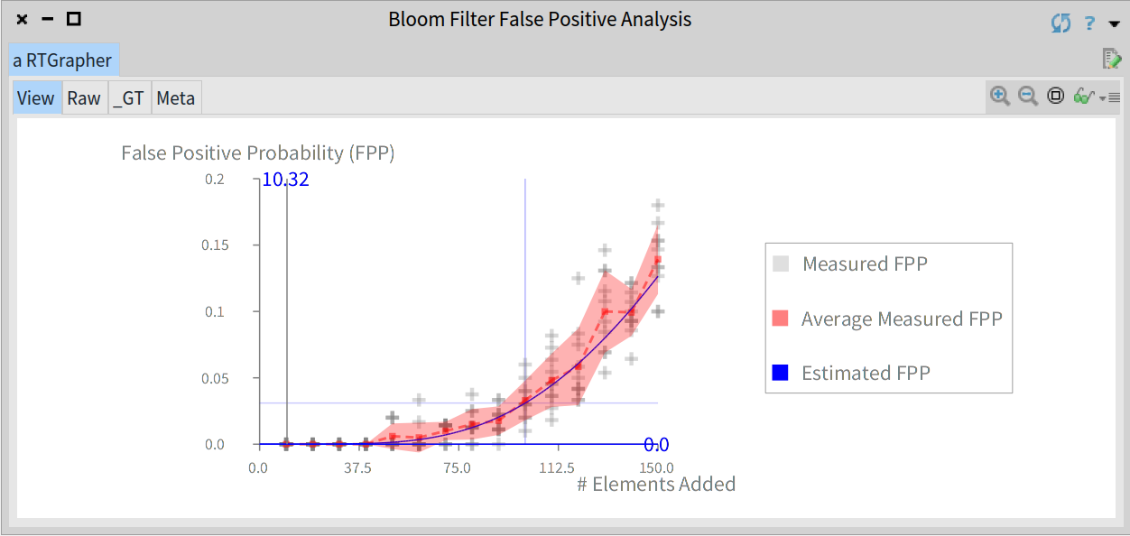
Graph showing the results for the empirical analysis of the Bloom filter's FPP
Benchmarking
A Bloom filter only requires a fixed number of k probes, so each insertion and search can be processed in O(k) time, which is considered constant.
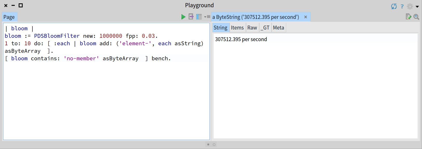
For instance, the following code will run a microbenchmark on the search operation for a Bloom filter previously populated with 10 elements and will show the number of operations executed per second:
Simple benchmarking for a Bloom filter with 10 elements
As the performance is constant, the result should be similar in the following case with the same Bloom filter containing 1 million elements previously added:
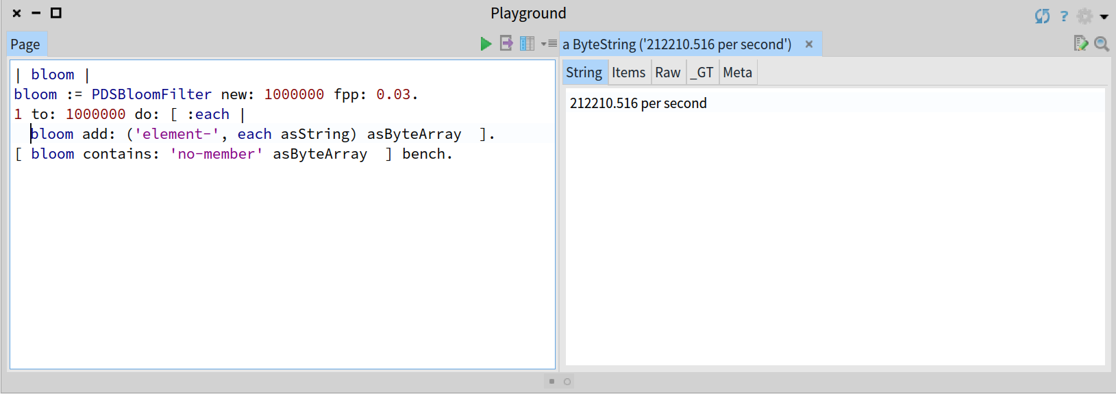
Simple benchmarking for the same Bloom filter with 1 million elements
A naive implementation based on a Collection data structure will show a linear O(n) performance, or in the best case of an ordered collection, a logarithmic O(log n) performance. In the following benchmarks you can check as the observed behaviour using an OrderedCollection degrades with the size of the collection (n):
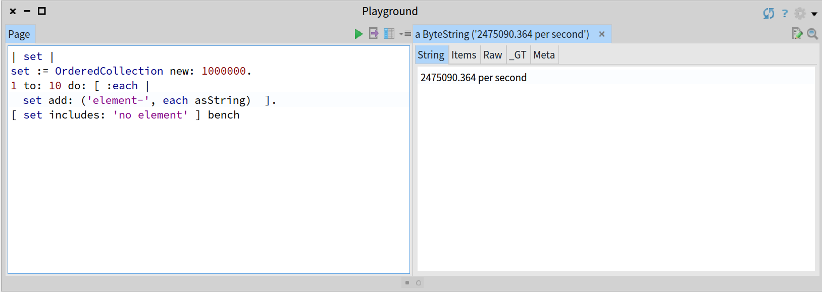
Simple benchmarking for an OrderedCollection with 10 elements
versus:
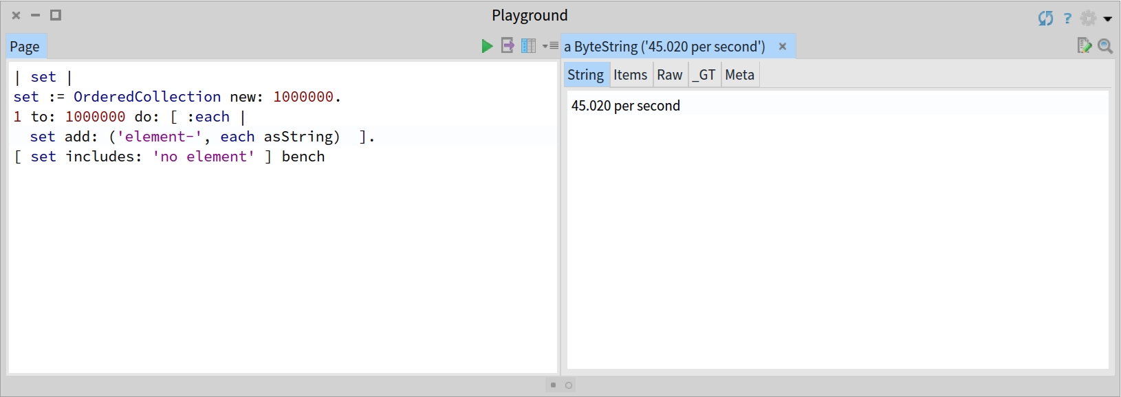
Simple benchmarking for and OrderedCollection with 1 million elements
Playground
PharoPDS provides a simple tool for the Bloom filter in order to allow you to explore and play with this data structure.
The PDSBloomFilterPlayground allows you to create Bloom filters to play with their operations and visualize them. You can even run benchmarks and profile them from the UI.
Let’s play with the playground running the following:
PDSBloomFilterPlayground open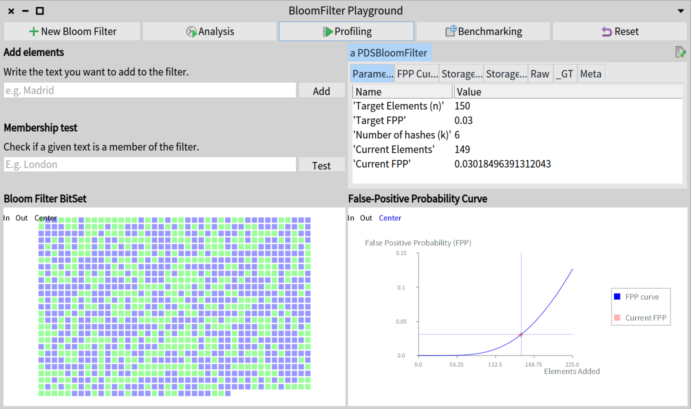
Custom playground tool to explore and play with Bloom filters
References
- On Probabilistic Data Structures:
- Burton H. Bloom. Space/Time Trace-offs in Hash Coding with Allowable Errors (1970).
- Donald E. Knuth. The Art of Computer Programming Volume 3: Sorting and Searching.
- Bloom Filters by Example.
- Andrii Gakhov, Probabilistic Data Structures and Algorithms for Big Data Applications.
- On Moldable Development:
- Andrei Chis’s PhD, “Moldable Tools” (2016). Available at http://scg.unibe.ch/archive/phd/chis-phd.pdf.
- Andrei Chis, “Playing with Face Detection in Pharo” (2018). Available at https://medium.com/@Chis_Andrei/playing-with-face-detection-in-pharo-e6dd297e0ca3.
- Tudor Girba, “Moldable Development” (2018). Available at https://www.youtube.com/watch?v=IcwHaF5aRTM.
Credits
- Header photo: Photo by kropekk_pl from pixaby.com with Pixabay License.